Matrices
By the end of this lesson, you’ll be able to:
- Represent data and transformations using matrices.
- Identify matrix dimensions and entries using row-column notation.
- Add, subtract, and scale matrices.
- Determine when matrix multiplication is possible.
- Multiply matrices using row-by-column multiplication.
- Interpret matrices in systems, transformations, and data contexts.
Key Ideas
A matrix is a rectangular array of numbers.
Example of a \(2 \times 3\) matrix:
\[ A= \begin{bmatrix} 1 & 4 & 2 \\ 3 & 0 & 5 \end{bmatrix} \]
Dimensions are written as:
\[ \text{rows} \times \text{columns} \]
So this matrix is a \(2 \times 3\) matrix because it has 2 rows and 3 columns.
- Row 1: \([1,\;4,\;2]\)
- Row 2: \([3,\;0,\;5]\)
Matrix Entries and Indices
Matrix entries are identified by their row and column positions.
For the matrix
\[ A= \begin{bmatrix} 1 & 4 & 2 \\ 3 & 0 & 5 \end{bmatrix} \]
we write
\[ a_{ij} = \text{entry in row }i,\text{ column }j. \]
The first index tells you the row.
The second index tells you the column.
Examples:
- \(a_{11}=1\)
- \(a_{12}=4\)
- \(a_{13}=2\)
- \(a_{21}=3\)
- \(a_{22}=0\)
- \(a_{23}=5\)
A helpful memory trick:
First index = row, second index = column.
For example:
\[ A= \begin{bmatrix} 1 & \boxed{4} & 2 \\ 3 & 0 & 5 \end{bmatrix} \qquad a_{12}=4 \]
because the boxed entry is in row 1, column 2.
Matrix Operations
Addition and Subtraction
Add or subtract corresponding entries.
This only works when matrices have the same dimensions.
\[ A+B=(a_{ij}+b_{ij}) \]
Scalar Multiplication
Multiply every entry by the scalar.
\[ kA=(ka_{ij}) \]
Matrix Multiplication
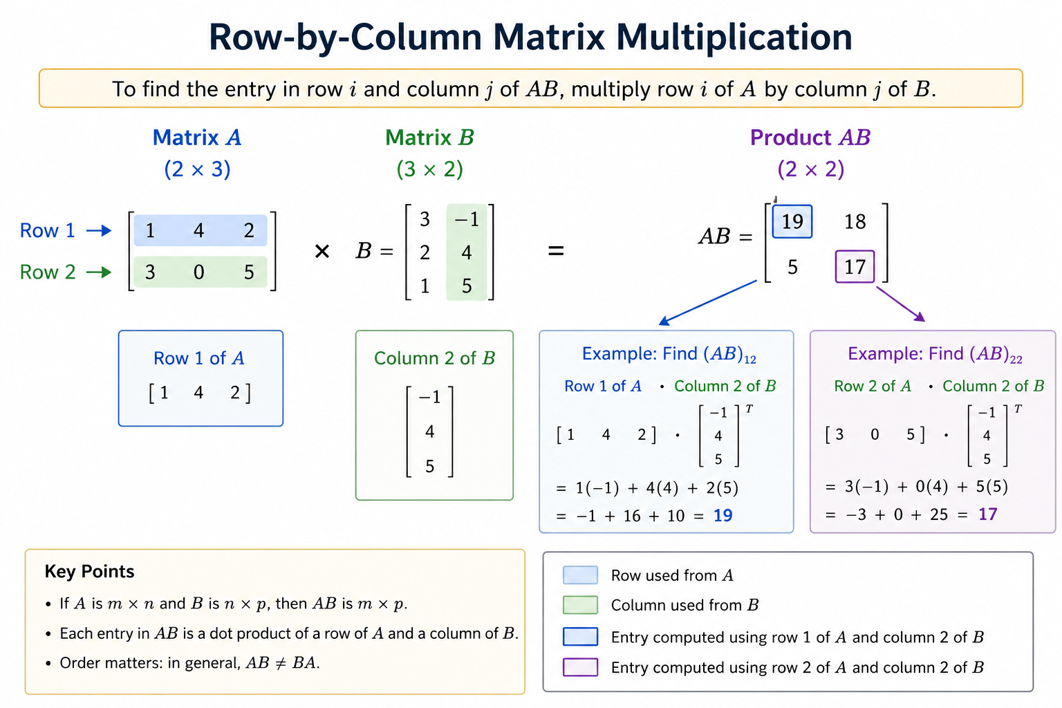
Matrix multiplication uses row-by-column multiplication.
The entry in row \(i\) and column \(j\) of the product matrix is found by multiplying row \(i\) of the first matrix by column \(j\) of the second matrix:
\[ (AB)_{ij} = \text{Row}_i(A)\cdot\text{Column}_j(B) \]
Matrix multiplication is not commutative:
\[ AB \ne BA \]
When Can Matrices Be Multiplied?
To multiply two matrices, the number of columns in the first matrix must equal the number of rows in the second matrix.
\[ (m\times n)(n\times p) \]
The two middle numbers must match.
Example:
\[ (2\times3)(3\times4) \]
Multiplication is possible because the inner dimensions match.
Example:
\[ (2\times3)(2\times4) \]
Multiplication is not possible because
\[ 3 \ne 2. \]
What Size Is the Product Matrix?
When matrix multiplication is possible:
\[ (m\times n)(n\times p) = (m\times p) \]
The product matrix keeps:
- The rows of the first matrix
- The columns of the second matrix
A useful visual is:
\[ \boxed{m}\times\cancel{n} \qquad \cancel{n}\times\boxed{p} = \boxed{m\times p} \]
Example:
\[ (2\times3)(3\times4) = 2\times4 \]
The resulting matrix has:
- 2 rows
- 4 columns
Common Problem Types
Adding or Subtracting Matrices
Addition and subtraction are only possible when dimensions match.
Example:
\[ \begin{bmatrix} 1 & 2\\ 3 & 4 \end{bmatrix} + \begin{bmatrix} 5 & 1\\ 0 & -2 \end{bmatrix} = \begin{bmatrix} 6 & 3\\ 3 & 2 \end{bmatrix} \]
Scalar Multiplication
Multiply every entry by the scalar.
Example:
\[ 2 \begin{bmatrix} 3 & -1\\ 4 & 2 \end{bmatrix} = \begin{bmatrix} 6 & -2\\ 8 & 4 \end{bmatrix} \]
Determining Whether Multiplication Is Possible
Suppose
\[ A \text{ is } 3\times2 \]
and
\[ B \text{ is } 2\times5. \]
Since the inner dimensions match,
\[ (3\times2)(2\times5) \]
multiplication is possible.
The product matrix will be
\[ 3\times5. \]
Matrix Multiplication: Row-by-Column
Multiply each row of the first matrix by each column of the second matrix.
Example:
\[ \begin{bmatrix} 1 & 2 \end{bmatrix} \begin{bmatrix} 3\\ 4 \end{bmatrix} = 1(3)+2(4) = 11 \]
This is a dot product: multiply corresponding entries and add.
Interpreting Matrices in Systems
A matrix can represent a system of linear equations.
Example:
\[ \begin{bmatrix} 2 & 1\\ 3 & -1 \end{bmatrix} \begin{bmatrix} x\\ y \end{bmatrix} = \begin{bmatrix} 5\\ 4 \end{bmatrix} \]
Represents:
- \(2x+y=5\)
- \(3x-y=4\)
Rows correspond to equations.
Columns correspond to variables.
Data Tables to Matrices
Matrices often store information from tables.
| Item | Price | Quantity |
|---|---|---|
| A | 3 | 4 |
| B | 5 | 2 |
Matrix form:
\[ \begin{bmatrix} 3 & 4\\ 5 & 2 \end{bmatrix} \]
In this setup:
- Row 1 represents Item A
- Row 2 represents Item B
- Column 1 represents price
- Column 2 represents quantity
Strategies
- Check dimensions before multiplying.
- The first index indicates the row; the second indicates the column.
- Make sure the inner dimensions match before multiplying.
- The product keeps the rows of the first matrix and columns of the second matrix.
- Use row-by-column multiplication carefully.
- For systems, rows correspond to equations and columns correspond to variables.
- When stuck, compute one entry at a time.
Worked Examples
Example 1 — Add Matrices
Compute:
\[ \begin{bmatrix} 4 & -1\\ 2 & 3 \end{bmatrix} + \begin{bmatrix} 1 & 5\\ 0 & -4 \end{bmatrix} \]
Add corresponding entries:
\[ \begin{bmatrix} 4+1 & -1+5\\ 2+0 & 3+(-4) \end{bmatrix} \]
Result:
\[ \begin{bmatrix} 5 & 4\\ 2 & -1 \end{bmatrix} \]
Example 2 — Scalar Multiplication
Compute:
\[ -3 \begin{bmatrix} 2 & -2\\ 1 & 4 \end{bmatrix} \]
Multiply every entry by \(-3\):
\[ \begin{bmatrix} -6 & 6\\ -3 & -12 \end{bmatrix} \]
Example 3 — Multiply Matrices
Compute:
\[ \begin{bmatrix} 2 & 1\\ 1 & 3 \end{bmatrix} \begin{bmatrix} 4 & 0\\ -2 & 5 \end{bmatrix} \]
First check dimensions:
\[ (2\times2)(2\times2) \rightarrow 2\times2 \]
Multiplication is possible.
First row × first column:
\[ 2(4)+1(-2)=6 \]
First row × second column:
\[ 2(0)+1(5)=5 \]
Second row × first column:
\[ 1(4)+3(-2)=-2 \]
Second row × second column:
\[ 1(0)+3(5)=15 \]
Result:
\[ \begin{bmatrix} 6 & 5\\ -2 & 15 \end{bmatrix} \]
Example 4 — System as a Matrix
System:
- \(3x+y=11\)
- \(x-2y=-3\)
Matrix form:
\[ \begin{bmatrix} 3 & 1\\ 1 & -2 \end{bmatrix} \begin{bmatrix} x\\ y \end{bmatrix} = \begin{bmatrix} 11\\ -3 \end{bmatrix} \]
The first row contains the coefficients of the first equation.
The second row contains the coefficients of the second equation.
- Reading \(a_{ij}\) as column first, row second.
- Trying to add or subtract matrices with different dimensions.
- Forgetting to check whether the inner dimensions match before multiplying.
- Forgetting that the product matrix keeps the rows of the first matrix and columns of the second matrix.
- Using element-by-element multiplication instead of row-by-column multiplication.
- Forgetting that \(AB \ne BA\).
- Mixing up rows and columns when forming system matrices.
- Arithmetic errors in matrix calculations.
Practice Problems
- Add:
\[ \begin{bmatrix} 1 & 2\\ 3 & 4 \end{bmatrix} + \begin{bmatrix} 4 & 0\\ -1 & 5 \end{bmatrix} \]
- Scalar multiply:
\[ 5 \begin{bmatrix} -2 & 3\\ 1 & 4 \end{bmatrix} \]
- Multiply:
\[ \begin{bmatrix} 1 & -1\\ 2 & 3 \end{bmatrix} \begin{bmatrix} 4\\ 5 \end{bmatrix} \]
- Write the system represented by:
\[ \begin{bmatrix} 2 & 3\\ -1 & 4 \end{bmatrix} \begin{bmatrix} x\\ y \end{bmatrix} = \begin{bmatrix} 7\\ 10 \end{bmatrix} \]
- For the matrix
\[ M= \begin{bmatrix} 8 & -2 & 5\\ 0 & 7 & 1 \end{bmatrix}, \]
find \(m_{23}\).
1.
\[ \begin{bmatrix} 5 & 2\\ 2 & 9 \end{bmatrix} \]
2.
\[ \begin{bmatrix} -10 & 15\\ 5 & 20 \end{bmatrix} \]
3.
\[ 1(4)+(-1)(5)=-1 \]
\[ 2(4)+3(5)=23 \]
Answer:
\[ \begin{bmatrix} -1\\ 23 \end{bmatrix} \]
4.
\[ 2x+3y=7 \]
\[ -x+4y=10 \]
5.
\(m_{23}\) means row 2, column 3.
The entry is
\[ 1. \]
Summary
- Matrices are rectangular arrays of numbers.
- Dimensions are written as rows × columns.
- Matrix entries use row-column notation: \(a_{ij}\) means row \(i\), column \(j\).
- Add and subtract matrices elementwise.
- Scalar multiplication multiplies every entry.
- Matrix multiplication uses row-by-column multiplication.
- To multiply matrices, the inner dimensions must match.
- The product matrix keeps the rows of the first matrix and columns of the second matrix.
- First index = row; second index = column.
- Check the inner dimensions before multiplying.
- The result keeps the outside dimensions.
- Matrix multiplication means row-by-column.
- If unsure, compute one entry at a time.