Graphing Systems of Equations
By the end of this lesson, you’ll be able to:
- Solve systems by graphing and locating intersection points.
- Identify whether a system has one solution, none, or infinitely many.
- Interpret graph-based systems that appear in real data or test-style problems.
Key Ideas
Graphing a system is all about understanding what the lines look like together.
A system can have:
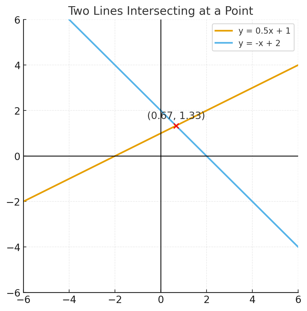
- One solution → lines intersect at a single point
- No solution → lines are parallel (same slope, different intercepts)
- Infinitely many solutions → lines are the same line
The easiest way to graph each equation is to first rewrite in slope-intercept form:
\[ y = mx + b \]
Then:
- Plot the y-intercept.
- Use slope (rise/run) to mark a second point.
- Draw both lines and look for the intersection.
Common Problem Types
Systems Already in Slope-Intercept Form
Just graph both lines directly.
Systems in Standard Form
Convert to \(y = mx + b\) first.
Systems With Parallel Lines
Same slope → immediately know “no solution.”
Systems That Coincide
When one equation is a multiple of the other.
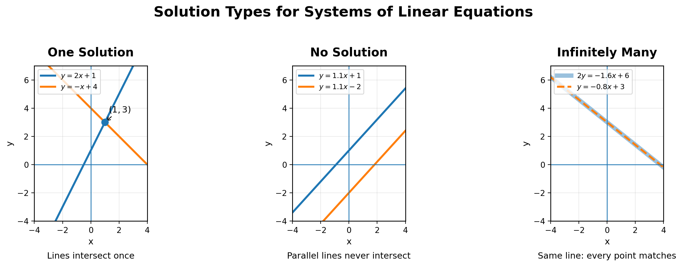
Before graphing, it helps to remember that every system falls into one of three categories:
- One solution → the lines intersect once.
- No solution → the lines are parallel.
- Infinitely many solutions → the equations represent the same line.
Strategies
- Always identify slopes first: it tells you immediately whether a solution exists.
- If equations are not in \(y = mx + b\), rewrite them—graphing becomes easier.
- Use a quick table of two points if slope-intercept form feels messy.
- When determining solution type, compare slopes and intercepts before graphing.
Worked Examples
Example 1 — Two Lines That Intersect
\[ \begin{cases} y = 2x + 1 \\ y = -x + 10 \end{cases} \]
Set equal to find intersection:
\[ 2x + 1 = -x + 10 \]
\[ 3x = 9 \Rightarrow x = 3 \]
Then:
\[ y = 2(3) + 1 = 7 \]
Solution: \((3, 7)\)
Example 2 — Parallel Lines (No Solution)
\[ \begin{split} & y = 3x + 4 \\ & y = 3x - 2 \end{split} \]
Same slope, different intercept → lines never meet.
Solution: no solution (parallel lines)
- Mis-reading slopes when converting to \(y = mx + b\).
- Plotting the intercept on the x-axis instead of the y-axis.
- Assuming two lines that “look close” must intersect—always check slope.
Practice Problems
Graph both equations and identify the solution:
\(y = x + 1\) and \(y = -x + 5\)Solve by graphing:
\(y = 2x - 3\)
\(2x - y = 6\)Determine whether the system has one solution, none, or infinitely many:
\(y = -4x + 7\)
\(4x + y = 2\)
1.
Set equal:
\(x + 1 = -x + 5\) → \(2x = 4\) → \(x = 2\)
\(y = 3\)
Solution: \((2, 3)\)
2.
Rewrite second equation:
\(2x - y = 6\) → \(-y = 6 - 2x\) → \(y = 2x - 6\)
Both lines have slope \(2\) but different intercepts → no solution
3.
Rewrite second: \(4x + y = 2\) → \(y = -4x + 2\)
Same slope as \(y = -4x + 7\) but different intercept → no solution
Summary
- A system’s solution corresponds to the intersection of two lines.
- Compare slopes first: equal slopes → no solution or infinite solutions.
- Graphing becomes easiest when using \(y = mx + b\).
- One intersection → one solution; no intersection → no solution.
- Convert to slope-intercept form before graphing.
- Compare slopes first to determine solution type quickly.
- Two lines with the same slope and same intercept represent the same line.
- Use rise/run to place points accurately—graphing errors cause incorrect conclusions.