Standard Deviation (Conceptual)
By the end of this lesson, you’ll be able to:
- Interpret standard deviation as a measure of spread around the mean.
- Compare the variability of datasets conceptually.
- Predict how shifting or scaling every value affects standard deviation.
- Explain how unusually distant values can affect standard deviation.
- Interpret standard deviation from simple graphs and real-world contexts.
Key Ideas
Standard deviation measures how spread out the values in a dataset are relative to the mean.
Conceptually:
- Small standard deviation → values tend to be close to the mean.
- Large standard deviation → values tend to be farther from the mean.
- Standard deviation is always:
\[ \boxed{SD\ge0} \]
- A dataset with no variation has:
\[ \boxed{SD=0} \]
You usually do not need to calculate standard deviation by hand in this lesson.
The important idea is:
\[ \boxed{\text{Standard deviation measures variability}} \]
Low vs. High Standard Deviation
Consider two datasets with the same mean:
\[ \text{Set A: }48,\ 49,\ 50,\ 51,\ 52 \]
and:
\[ \text{Set B: }20,\ 35,\ 50,\ 65,\ 80 \]
Both have mean:
\[ 50 \]
But Set A is tightly clustered around 50, while Set B is much more spread out.
Therefore:
\[ \boxed{SD_B>SD_A} \]
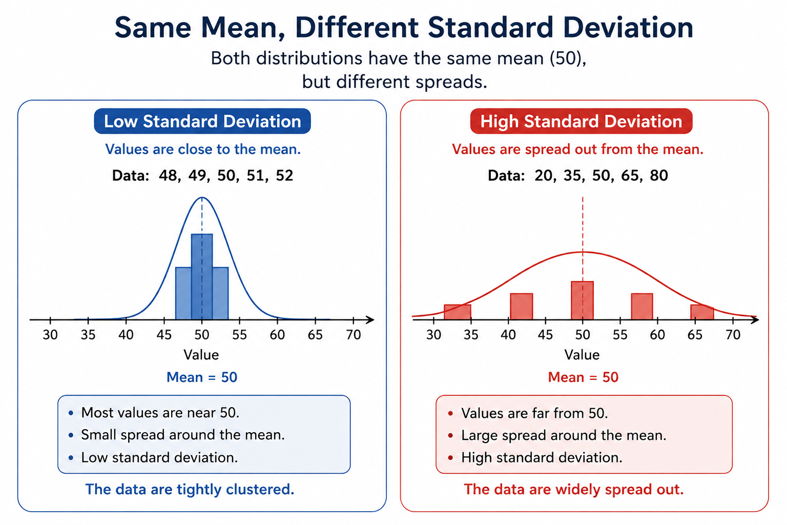
Two datasets can have the same mean but very different standard deviations.
The mean tells you about the center.
Standard deviation tells you about the spread around that center.
What Does a Standard Deviation of Zero Mean?
Suppose the data are:
\[ 7,\ 7,\ 7,\ 7 \]
The mean is:
\[ 7 \]
Every observation is exactly equal to the mean.
There is no spread at all.
Therefore:
\[ \boxed{SD=0} \]
Any dataset containing variation must have a standard deviation greater than 0.
How Changes Affect Standard Deviation
Certain transformations have predictable effects on standard deviation.
Adding or Subtracting a Constant
Suppose:
\[ 3,\ 7,\ 9 \]
becomes:
\[ 13,\ 17,\ 19 \]
because 10 was added to every value.
Every value moves 10 units to the right, and the mean also moves 10 units to the right.
But the distances between the values do not change.
Therefore:
\[ \boxed{\text{SD stays the same}} \]
In general, adding or subtracting the same constant from every observation does not change standard deviation.
Multiplying by a Constant
Suppose:
\[ 5,\ 6,\ 7 \]
is multiplied by 3:
\[ 15,\ 18,\ 21 \]
All distances are now 3 times as large.
Therefore:
\[ \boxed{\text{SD is multiplied by }3} \]
In general, if every value is multiplied by \(k\):
\[ \boxed{ SD_{\text{new}}=|k|SD_{\text{old}} } \]
The absolute value is important because standard deviation cannot be negative.
For example, multiplying every value by \(-2\) makes the standard deviation:
\[ \boxed{2\text{ times as large}} \]
Adding an Extreme Value
Consider:
\[ 10,\ 11,\ 12 \]
The observations are close together.
Now consider:
\[ 10,\ 11,\ 12,\ 100 \]
The value 100 lies very far from the other observations and from the new mean.
This makes the data much more spread out.
Therefore, in this example:
\[ \boxed{\text{standard deviation increases substantially}} \]
Extreme observations often have a strong effect on standard deviation because SD is sensitive to how far observations lie from the mean.
Common Problem Types
1. Comparing Spread From Data Lists
You may be given two datasets and asked which has the larger standard deviation.
For example:
\[ A: 49,\ 50,\ 51 \]
\[ B: 20,\ 50,\ 80 \]
Both have mean 50.
Set A stays very close to the mean.
Set B contains observations much farther from the mean.
Therefore:
\[ \boxed{\text{Set B has the larger standard deviation}} \]
2. Comparing Datasets With Different Means
The dataset with the larger mean does not necessarily have the larger standard deviation.
Consider:
\[ A: 98,\ 100,\ 102 \]
and:
\[ B: 8,\ 10,\ 12 \]
Their means are different:
\[ 100\quad\text{and}\quad10 \]
but their spreads are identical.
Each dataset has values:
\[ 2\text{ below the mean},\quad \text{at the mean},\quad 2\text{ above the mean} \]
Therefore, they have the same standard deviation.
\[ \boxed{SD_A=SD_B} \]
3. Shifting Every Value
Suppose every score in a dataset increases by 7 points.
The mean also increases by 7.
However, the distances of the observations from the mean remain unchanged.
Therefore:
\[ \boxed{\text{SD does not change}} \]
4. Scaling Every Value
Suppose every measurement is multiplied by 4.
Then all distances from the mean become 4 times as large.
Therefore:
\[ \boxed{\text{SD is multiplied by }4} \]
5. Effects of Extreme Values
Compare:
\[ 5,\ 6,\ 7 \]
with:
\[ 5,\ 6,\ 7,\ 100 \]
The second dataset contains an observation far from the others.
Its spread is much greater.
Therefore, its standard deviation is much larger.
6. Comparing Distributions From Graphs
When two graphs use the same horizontal scale, a distribution whose observations are concentrated near the center generally has a smaller standard deviation than one whose observations are spread farther from the center.
For example:
- narrow cluster → smaller SD
- broad spread → larger SD
However, look at the entire distribution, not only its range.
A boxplot does not show standard deviation directly.
A larger box means a larger interquartile range (IQR), but that does not automatically prove that the standard deviation is larger.
Use boxplots to compare spread broadly, but do not treat IQR and standard deviation as interchangeable.
7. Comparing Consistency
Standard deviation can also describe consistency.
Suppose two athletes have the same average score:
- Athlete A’s scores stay close to the average.
- Athlete B’s scores vary widely from game to game.
Athlete A has the smaller standard deviation.
Therefore, Athlete A is more consistent.
This interpretation appears frequently in real-world statistics problems.
Strategies
- Focus on distances from the mean, not simply the size of the values.
- Tightly clustered observations → smaller SD.
- Widely scattered observations → larger SD.
- Do not assume a larger mean means a larger SD.
- Adding or subtracting the same constant from every value → SD unchanged.
- Multiplying every value by \(k\) → SD multiplied by \(|k|\).
- Extreme observations can greatly increase spread.
- If all observations are identical → SD = 0.
- When comparing graphs, make sure the horizontal scales are comparable.
- Think smaller SD = more consistency when interpreting repeated measurements.
Worked Examples
Example 1 — Compare Two Datasets
Which dataset has the larger standard deviation?
\[ A: 49,\ 50,\ 50,\ 51 \]
\[ B: 20,\ 40,\ 60,\ 80 \]
Set A is tightly clustered.
Its values are all near 50.
Set B spans from:
\[ 20\text{ to }80 \]
and its values are much farther apart.
Therefore:
\[ \boxed{\text{Set B has the larger standard deviation}} \]
Example 2 — Shift Every Value
Consider:
\[ 4,\ 8,\ 12 \]
Now add 10 to every value:
\[ 14,\ 18,\ 22 \]
The original values are separated by:
\[ 4 \]
and:
\[ 4 \]
The new values have exactly the same spacing.
The entire dataset has simply shifted to the right.
Therefore:
\[ \boxed{\text{standard deviation stays the same}} \]
Example 3 — Multiply Every Value
Consider:
\[ 5,\ 6,\ 7 \]
Now multiply every value by 3:
\[ 15,\ 18,\ 21 \]
Originally, the values are spaced 1 unit apart.
After scaling, they are spaced 3 units apart.
All distances from the mean are multiplied by 3.
Therefore:
\[ \boxed{ SD_{\text{new}}=3SD_{\text{old}} } \]
Example 4 — Multiply by a Negative Number
A dataset has standard deviation:
\[ SD=5 \]
Every value is multiplied by:
\[ -2 \]
Use:
\[ SD_{\text{new}} = |k|SD_{\text{old}} \]
So:
\[ SD_{\text{new}} = |-2|(5) \]
\[ =2(5) \]
\[ \boxed{10} \]
The negative sign reverses the ordering of the data but does not create a negative standard deviation.
Example 5 — Introduce an Extreme Value
Consider:
\[ 10,\ 11,\ 12 \]
These observations are close together.
Now add:
\[ 100 \]
giving:
\[ 10,\ 11,\ 12,\ 100 \]
The value 100 lies very far from the rest of the data.
The overall spread becomes much greater.
Therefore:
\[ \boxed{\text{standard deviation increases substantially}} \]
Example 6 — Same Spread, Different Center
Compare:
\[ A: 8,\ 10,\ 12 \]
and:
\[ B: 98,\ 100,\ 102 \]
Set B can be obtained by adding 90 to every value in Set A:
\[ 8+90=98 \]
\[ 10+90=100 \]
\[ 12+90=102 \]
Adding a constant changes the mean but not the spread.
Therefore:
\[ \boxed{SD_A=SD_B} \]
- Assuming the dataset with the larger mean must have the larger standard deviation.
- Thinking that adding a constant changes standard deviation.
- Forgetting that multiplying by \(k\) multiplies SD by \(|k|\).
- Thinking a negative multiplier produces a negative standard deviation.
- Assuming equal ranges guarantee equal standard deviations.
- Using only the maximum and minimum to judge standard deviation when the rest of the distributions differ.
- Treating IQR and standard deviation as the same measure of spread.
- Forgetting that a dataset with identical values has standard deviation 0.
Practice Problems
- Which dataset has the larger standard deviation?
\[ A: 9,\ 10,\ 11 \]
\[ B: 3,\ 20,\ 37 \]
Every value in a dataset is increased by 7. What happens to the standard deviation?
Every value in a dataset is multiplied by \(-2\). What happens to the standard deviation?
Compare:
\[ A: 48,\ 50,\ 52 \]
\[ B: 98,\ 100,\ 102 \]
Which has the larger standard deviation?
A dataset has standard deviation 6. Every value is multiplied by 4. What is the new standard deviation?
What is the standard deviation of:
\[ 12,\ 12,\ 12,\ 12,\ 12 \]
- Two basketball players have the same mean number of points per game. Player A’s scores stay very close to the mean, while Player B’s scores vary widely. Which player has the smaller standard deviation?
1. Compare how spread out the values are.
Set A:
\[ 9,\ 10,\ 11 \]
is tightly clustered around 10.
Set B:
\[ 3,\ 20,\ 37 \]
is much more spread out around 20.
Therefore:
\[ \boxed{\text{Set B has the larger standard deviation}} \]
2. Adding 7 shifts every value by the same amount.
The mean also shifts by 7, so the distances from the mean do not change.
Therefore:
\[ \boxed{\text{SD stays the same}} \]
3. If every value is multiplied by \(k\), standard deviation is multiplied by:
\[ |k| \]
Here:
\[ k=-2 \]
so:
\[ |-2|=2 \]
Therefore:
\[ \boxed{\text{SD doubles}} \]
4. Compare:
\[ 48,\ 50,\ 52 \]
and:
\[ 98,\ 100,\ 102 \]
The second dataset is obtained by adding 50 to every value in the first.
Adding a constant changes the center but not the spread.
Therefore:
\[ \boxed{\text{The two datasets have the same standard deviation}} \]
5. The original standard deviation is:
\[ 6 \]
Every value is multiplied by:
\[ 4 \]
Therefore:
\[ SD_{\text{new}} = 4(6) \]
\[ \boxed{24} \]
6. Every value is identical:
\[ 12,\ 12,\ 12,\ 12,\ 12 \]
The mean is 12, and every observation is exactly equal to the mean.
There is no spread.
Therefore:
\[ \boxed{SD=0} \]
7. Player A’s scores stay closer to the mean.
That means Player A’s scores have less variability.
Therefore:
\[ \boxed{\text{Player A has the smaller standard deviation}} \]
Player A is also the more consistent scorer.
Summary
Standard deviation measures how spread out observations are around their mean.
- Smaller SD → values are more tightly clustered.
- Larger SD → values are more widely spread.
- No variation → \(SD=0\).
- Adding or subtracting a constant:
\[ \boxed{\text{does not change SD}} \]
- Multiplying every value by \(k\):
\[ \boxed{ SD_{\text{new}}=|k|SD_{\text{old}} } \]
- Extreme observations can strongly increase standard deviation.
- Mean describes center; standard deviation describes spread.
- A smaller standard deviation often indicates greater consistency.
- Tight cluster → small SD.
- Wide spread → large SD.
- Same mean does not mean same SD.
- Different means can still have the same SD.
- Add/subtract a constant → SD unchanged.
- Multiply by \(k\) → SD × \(|k|\).
- All values equal → SD = 0.
- More consistent → smaller SD.